

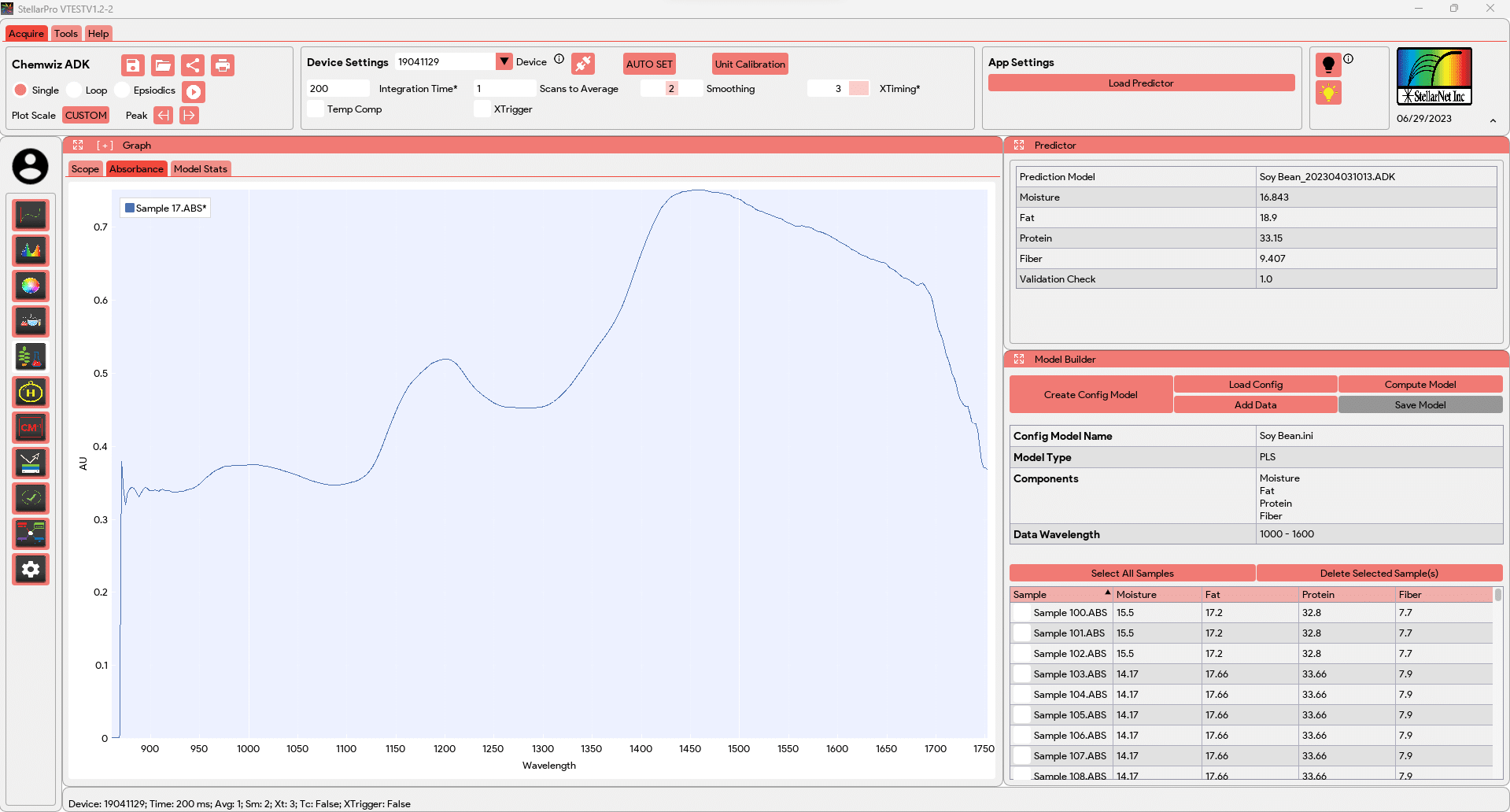
The ChemWiz ADK App utilizes spectrometric absorbance data to predict and classify the composition of a sample using advanced techniques such as Partial Least Squares (PLS) and Nearest Neighbor for classification. It employs multivariate analysis methods to analyze the complex absorbance patterns and extract meaningful information about the sample’s composition.
The app offers a built-in predictor that allows users to input absorbance data and obtain predictions for the composition of the sample. This provides a quick and convenient way to obtain insights about the sample without the need for extensive data analysis.
Additionally, the app includes an advanced model builder, which enables users to create customized models using their own data. The model builder provides a comprehensive set of tools and algorithms to optimize and refine the predictive models based on specific requirements and applications.
App Settings
![]() The App Setting in the Chemwiz ADK App includes a “Load Predictor” button, which allows users to load a pre-built model (ADK/ADKc files) into the predictor. By clicking the “Load Predictor” button and selecting the appropriate model file, users can load the trained model into the predictor. This model contains all the necessary parameters, weights, biases, and regression coefficients that were previously trained and optimized using absorbance data. Once the model is loaded, it becomes ready to make predictions on the classification or perform quantitative analysis of the composition of a sample based on the measured absorbance data. The details of the loaded predictor model can be viewed in the “Model Stats” tab in the Graph window and in the Predictor window.
The App Setting in the Chemwiz ADK App includes a “Load Predictor” button, which allows users to load a pre-built model (ADK/ADKc files) into the predictor. By clicking the “Load Predictor” button and selecting the appropriate model file, users can load the trained model into the predictor. This model contains all the necessary parameters, weights, biases, and regression coefficients that were previously trained and optimized using absorbance data. Once the model is loaded, it becomes ready to make predictions on the classification or perform quantitative analysis of the composition of a sample based on the measured absorbance data. The details of the loaded predictor model can be viewed in the “Model Stats” tab in the Graph window and in the Predictor window.
Windows
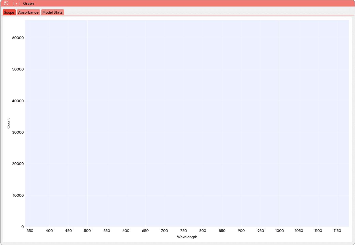
- The Graph window in the Chemwiz ADK App includes a Scope plot that provides real-time visualization of the spectrometric absorbance data. It also features an Absorbance plot, which displays the absorbance values across the specified wavelengths.
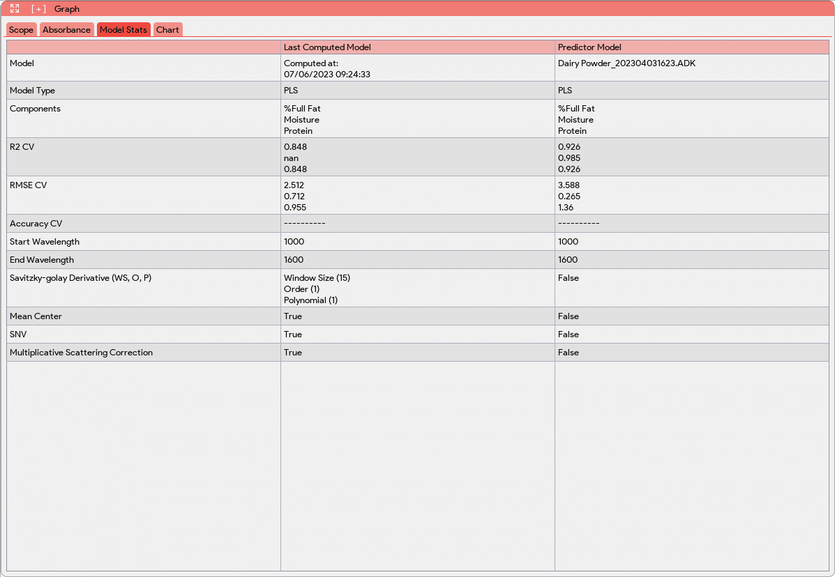
In addition to the graphs, the Graph window includes a Model Stats tab. This tab presents various information about the loaded model, including the model name, type, and the names of its components. It also provides evaluation metrics such as R2 (coefficient of determination) and RMSE (root mean square error), which assess the performance of the model. The Model Stats tab further presents the processing steps applied to the absorbance data during the modeling process. This gives users insights into the data pre-processing techniques employed to optimize the model’s performance. The Model Stats tab also allows the users to compare the loaded model with pre-existing models. This comparison assists users in making informed decisions about which model to use in production or for further analysis.
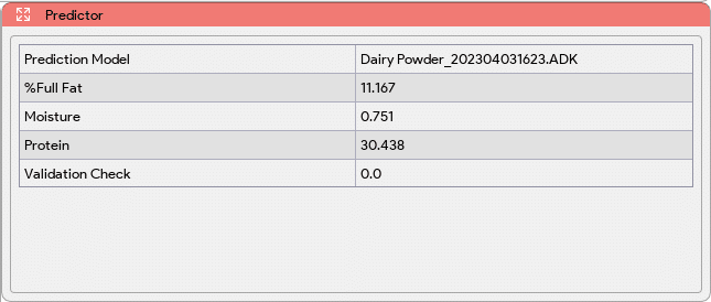
- The Predictor window continuously monitors and processes the incoming spectrometric data to perform predictions using the loaded model. This real-time analysis allows for efficient and timely prediction of the composition or concentration of the components in the sample.
- The Model Builder window in the Chemwiz ADK App offers a comprehensive set of tools and options to create either a Partial Least Squares (PLS) regression model or a classification model using absorbance data and known component concentration.
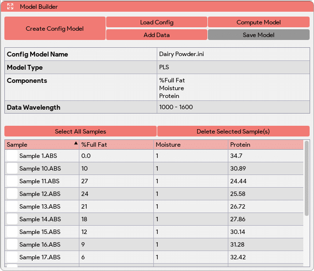
Within the Model Builder window, users can access various functionalities and settings to build their models:
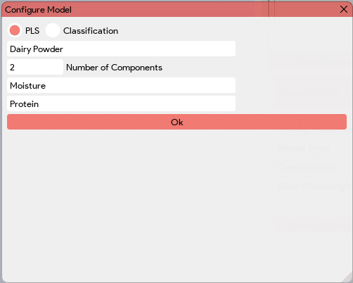
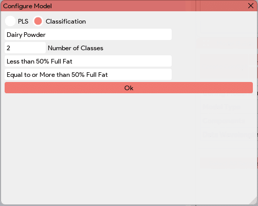
 The “Create Config Model” button in the Model Builder window allows users to generate a folder (located in the “StellarPro Data” folder) and a configuration file (.ini) for the model. The configuration file contains essential information such as the model type (quantitative/qualitative), model name, number of components/classes, and their names. It is used to store details about the model before it is built, serving as a reference for subsequent steps in the model building process.
| PLS
|
Classification
|
 The “Load Config” button in the Model Builder window enables users to load an existing configuration file. This feature is particularly useful when users want to create multiple models for the same data and model type. By loading a saved configuration file, users can quickly access and utilize the predefined model settings, including the model type, name, number of components, and component names. This allows for efficient model creation and facilitates the comparison and analysis of different models based on the same data.
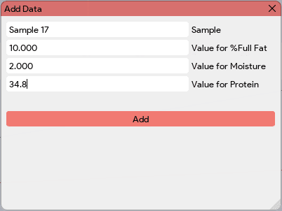
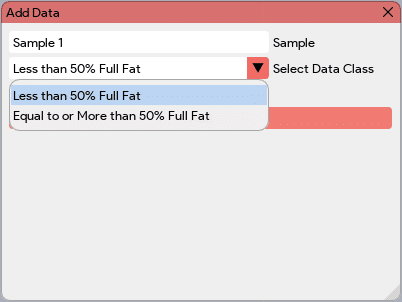
 The “Add Data” button in the Model Builder window allows users to incorporate the latest absorbance readings into the data table for model building. By clicking this button, users can add the absorbance values for the sample under consideration. Additionally, the application prompts users to input the known concentrations for the corresponding components (PLS) or class label (classification) associated with the absorbance readings. At the end of the Model Builder window, all the added samples or data, along with their corresponding component values, will be displayed in a table. This table provides a comprehensive overview of the data used for model building.
| PLS
|
Classification
|
 The “Compute Model” button in the Model Builder window triggers a window where users can select various preprocessing steps for data cleaning, augmentation, and feature enhancement. These steps may include techniques like derivative, mean centering, standard normal variate filtering (SNVF), and multiplicative scatter correction (MSC).
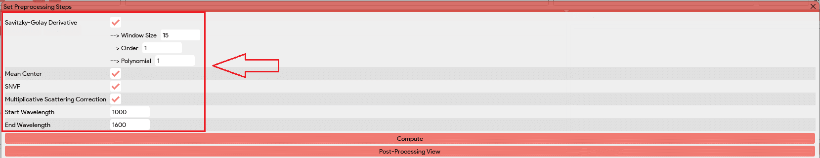
Upon selecting the desired preprocessing steps, users have the option “Post-Processing View” to visualize the data after these steps are applied. This allows them to assess the impact of the preprocessing techniques on the data and make informed decisions about the suitability of the chosen steps.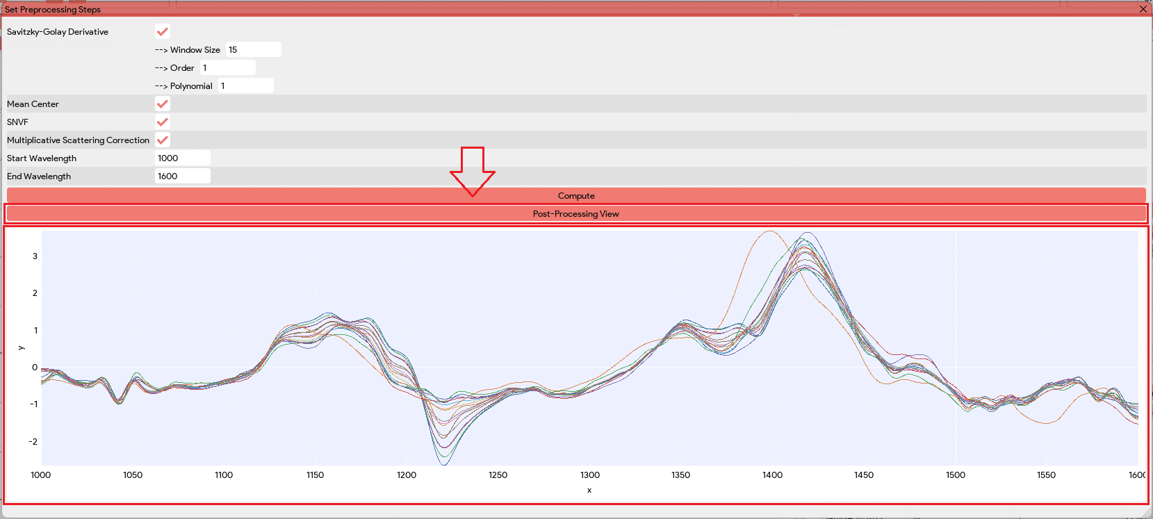
When the “Compute Model” button is clicked, the application applies the selected preprocessing steps to the data and creates a model based on the configuration specified earlier. The model’s evaluation metrics, such as R2 (coefficient of determination) and RMSE (root mean square error), are then populated in the Model Stats tab. These metrics provide valuable insights into the performance and predictive capabilities of the model, allowing users to evaluate and assess its effectiveness.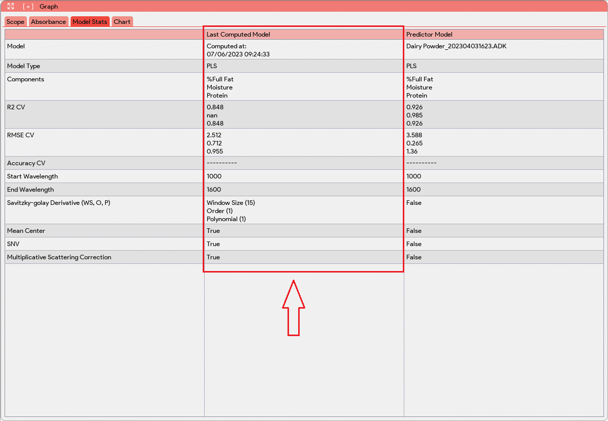
Additionally, a new tab “Chart” will be added to the Graph Window. This new tab will provide visual representations of the model’s performance. In this Chart tab, the PLS model will generate plots that compare the actual values versus the predictions for each component using cross-validation data. These plots allow users to assess how well the model predicts the component concentrations or classifications. For classification models, the Chart tab will display a confusion matrix. The confusion matrix displays the classification results, showing the number of samples correctly classified and misclassified for each class. This matrix provides a comprehensive overview of the model’s accuracy and performance in classifying different samples.
PLS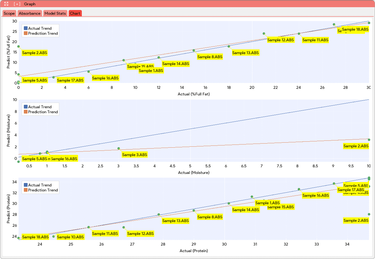 |
Classification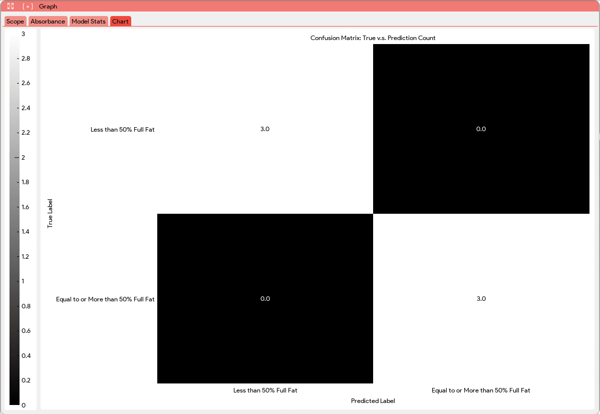 |
After the computation process, the application performs outlier detection using residual and leverage outlier detection methods. Outliers are data points that deviate significantly from the expected pattern or trend. The application will automatically detect these outliers and highlight them red in the table, making them easily identifiable. The identification of outliers allows users to assess the impact of these data points on the model’s performance and reliability. Depending on the user’s discretion and the specific requirements of the model, they can choose to delete the outlier data points or consider retaking those measurements to ensure a robust model building process.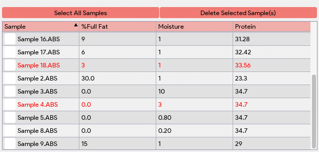
 A desired predictor model can be saved by clicking on the “Save Model” button, and a file browser will prompt the user to select the store location and enter the predictor name to save.